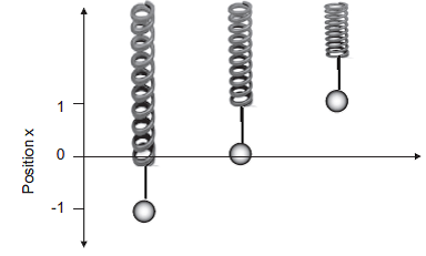
Change is an elementary phenomenon in life. It is most visible in movement of matter. It is useful to look at a simple, well observable and controllable system: a mass m at the end of a spring. It is the classical model of linear elasticity, associated with the 17th-century British scholar Hooke. Change is in this case about potential and kinetic energy in a gravitational field.
Assume that the position of the mass is indicated with and that initially it is at rest in position
. If you pull the mass, it starts an oscillating movement (Figure 1a). This happens under the influence of two forces: the gravitational force Fg and the spring force Fs. The gravitational force is given by Fg = mg with g the gravitational constant in m/
, and the spring force is approximated by Fs = −kx with k the spring constant in kg/
. In the rest position, the gravitational force pulls the mass a small distance down – say xR, at which the two forces are equal: Fg = Fs and m.g = k.xR or xR = m.g/k. Let us normalise and define xR = 0. Suppose you pull down the mass to a position – p at time t = 0. At this point the upward spring force will equal Fs = kp and the potential energy in the gravitational field has dropped with an amount of mgp. The system is in equilibrium because your hand exerts a downward force equal to Fs − Fg.
Letting loose, the mass will start to move upward because of Fs – Fg = kp. Its velocity v increases and the kinetic energy is ½mv2. The law of conservation of energy implies that the sum of potential and kinetic energy remains constant. Therefore, when the mass passes in its upward movement the point x = 0, the potential energy it had at x = p, equal to mgp, has been converted into kinetic energy (assuming an perfectly isolated spring). Hence, at mgp = ½mv2 or v = gp on passing the point xR . The further you pull the mass down, the greater the speed at which the mass goes past the point xR.
Using the formal language of mathematics, one can approximate the movement of a mass on a spring with two differential equations:
dx/dt = v (1a) (1b)
in which the small d indicates an infinitesimally small change. The first one says that the velocity v equals the rate of change of displacement and the second one that the rate of change of velocity, that is, the acceleration, is negatively proportional to the distance from the point x(0) = xR = 0. Substituting the first equation into the second yields a single second-order differential equation which can be solved analytically . I will not derive analytical solutions and instead use the simulation software package Stella® to explore the system behaviour over time. The harmonic oscillations in Figure 1a represent the position of a mass, x(t), over time for the (ideal) frictionless spring. Plotting the velocity of the mass, v(t) = dx(t)/dt, as a function of the position x(t), one gets the phase diagram (Figure 1b).
Of course, you know that the mass will not keep oscillating forever. There will be friction, which shows up as a dampening force proportional to the velocity. This yields an additional term in the expression for the restoring force:
dx/dt = v (2a) (2b)
with r the friction coefficient. This description is more realistic because it incorporates the phenomenon that any process is irreversible and more ordered energy is dissipated into heat (molecular motion) in agreement with the second law of thermodynamics. The speed of the mass slowly diminishes over time and ends in the equilibrium point x(0) = xR = 0, called the attractor (Figure 1c–d). One can also apply an external force on the mass, for instance, by pulling it at a constant frequency ω and amplitude q. Now, the natural and the forced movement interact and the position x(t) over time becomes erratic (Figure 1e–f). If someone would show you this graph, you would have a hard time to discover how simple the underlying system actually is!
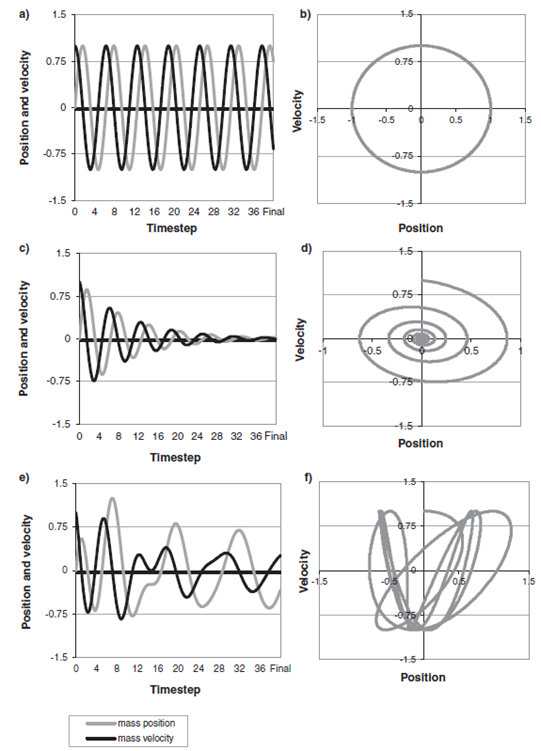
Figure 1a-f. Idealized movements of a mass at the end of a spring.
What happens if the spring constant is itself a function of the displacement from equilibrium: k = k(x)? Suppose it is found that the spring constant behaves according to k = ( – 1). This implies that the system behaves like a mass at the end of a spring only for x > 1 or x < −1. For −1 < x < 1 the value of k is negative and the system operates in this domain not with deceleration due to friction but with acceleration. In system dynamics terms, there is a positive or amplifying feedback in this domain. Such a system is described by the two differential equations:
dx/dt = v (3a) (3b)
The system has three attractors, two stable and one unstable. A steel spring placed between two permanent magnets is a bistable oscillator described by these equations (Bossel 1994). If there is no dampening (r = 0), the system oscillates between the two attractors, as shown in the trajectory in time and in the phase diagram in Figure 1g–h. The damped system moves towards one of the two attractors, but it is hard to say in advance to which one. A slight uncertainty or change in the initial state, that is, x at t = 0, or in one of the parameters can make the system move towards a different equilibrium state – it is extremely sensitive to the initial conditions. The term ( – 1) introduces a nonlinearity. This usually leads to multiple equilibria and critical dependence on the initial conditions. These simple technical devices show complex behaviour.
If this system is also subjected to an external force of constant frequency ω and amplitude q:
dx/dt = v (4a) (4b)
its behaviour becomes irregular and even chaotic for certain parameter domains (Figure 2a-f). Chaotic means in this context that the system – the same steel spring but placed now in an oscillating, not a permanent magnetic field – behaves deterministically but is nevertheless unpredictable in the sense that its future can only be known if one would know the initial state with infinite precision. Note that these equations describe the movement of a mass in space and time (potential and kinetic energy) and not the associated heat flow (friction).
These simulations show that rather simple nonlinear equations (‘models’), which may or may not be accurate descriptions of real-world systems, can exhibit complex behaviour over time. Their use as analogues is useful in the sustainability discourse, provided that one understands the idealising assumptions. In particular, the investigation of multiple equilibria in ecosystems and economic systems is a new area of research. Elementary chemical processes, for instance, chemical kinetics, provide more interesting and complex examples, but this is considered beyond the scope of this book. I refer the reader to the suggested literature.
Leave A Comment