In the context of sustainable development, the emphasis is usually on depletion and a key question is: How big is the resource or, in expert jargon, what is the geological resource base? First, I look at mineral ores. Solid evidence on resource ore quantity and quality is limited by its very nature to those regions that have been explored. However, it is possible to infer more speculative occurrences with hypotheses about how ores have formed in geological time. In 1954, the geologist Ahrens proposed a ‘fundamental law of geochemistry’: The concentration or grade of an element is lognormally distributed in a specific igneous rock. This – not uncontroversial – crustal abundance geostatistical (CAG) model makes it possible to estimate the geological resource in the form of a grade distribution curve. This is important because the extraction cost, in money and energy units, is to a large extent determined by the ore grade. The outcome of such an estimation is the lognormal distribution shown in Figure 1 for the relatively abundant elements titanium (Ti) and lead (Pb) and the very rare element mercury (Hg).
The ‘fundamental law of geochemistry’, proposed by Ahrens in 1954, is: The concentration of an element is lognormally distributed in a specific igneous rock. The so-called Crustal Abundance Geostatistical (CAG) model assumes that:
- Ore deposit formation processes (igneous activity, erosion-sedimentation, solution-precipitation) are sequences of separation steps
- Upon each step, a mass of M units of material with average concentration Gav is divided into two equal parts, one enriched, one depleted
With TotalMass TM conserved and q the specific mineralizability, an indicator of the efficiency of the separating process (0<q<1), the enrichment/depletion after one step is:
![]() After b naturally occurring ‘separating steps’, the total mass TM is:
After b naturally occurring ‘separating steps’, the total mass TM is:
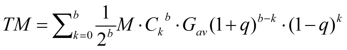 The amount of metal in class k, Mk, can be calculated with the formula for a binomial distribution, which represents a continuous – for hundreds of millions of years – mixing of elements:with Ckb the binomial coefficient and (1/2b)M the unit deposit size after b separating steps. Natural processes, fed by solar and nuclear energy, did the separating work!
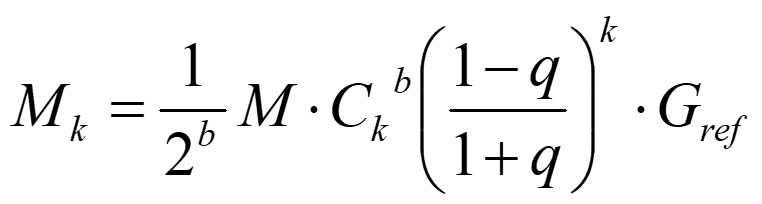 with Gref the grade of the richest occurring ore, M the total earth crustal mass, Ckb the binomial coefficient and q the element-specific mineralizability factor. For more details I refer to the literature.
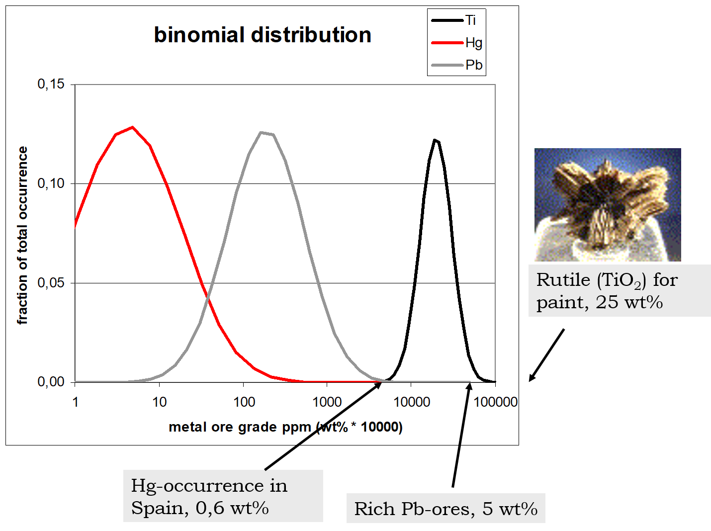 Figure 1. The frequency distribution (binomial) of three elements in the Earth’s crust as calculated with the CAG model. The curves depict the fraction of the estimated total amount at a given concentration interval. The arrows indicate present average ore concentration for Titanium (Ti), lead (Pb) and mercury (Hg).
The CAG model can put resource scarcity in a long-term perspective. For instance, a news item such as ‘China’s export restraints on rare earth elements has inflamed trade ties’ is clearly to be interpreted in a short-term market and trade perspective and not (yet) considered a long-term scarcity concern. But there are at least two caveats. First, the analysis does not include elements in seawater. Although the concentrations are low, the amounts are huge (Table 1). Second, the evidence from mining metal ores up to now does not exclude the possibility that, for chemical or physical reasons, the distribution differs from a binomial one. It can turn out to be a bimodal one, which means that the distribution shows two maxima because the element is not concentrated in a particular range. Such a bimodal distribution would lead to a very different estimate of the amounts of metal available at low concentrations.
| Table 1. Estimates of average metal abundance in crust and seawater, of total mobilisation flows and the anthropogenic fraction therein.a Also, indications of richest ore and specific mineralisability are given.b The elements for which the distribution is drawn in Figure 13.4 are shown in bold. | ||||||
| Avg conc in ppm | Total mobilisation rate (TMR) Tg/yr | Anthropogenic fraction in TMR % of total | Richest ore grade in crust wt % | q spec mineralisability | ||
| Metal | crust g/Mg (ppm) | Seawater g/Mg (ppm) | ||||
| Aluminum (Al) | 77,440 | 0.002 | 309 | 26 | 49.2 | 0.041 |
| Iron (Fe) | 30,890 | 0,002 | 848 | 90 | 0.087 | |
| Magnesium (Mg) | 13,510 | 1,290 | 1,944 | 3 | ||
| Carbon (C) | 3,240 | 28 | 118,450 | 9 | ||
| Titanium (Ti) | 3,117 | – | 11 | 54 | 24.7 | 0.127 |
| Sulphur (S) | 953 | 905 | 766 | 22 | ||
| Phosphorous (P) | 665 | 0,1 | 538 | 6 | ||
| Chlor (Cl) | 640 | 19,354 | 6,264 | 2 | ||
| Manganese (Mn) | 527 | 0.0002 | 40 | 22 | 43.7 | 0.201 |
| Zirconium (Zr) | 237 | – | 1.6 | 78 | ||
| Nitrogen (N) | 83 | 150 | 6,067 | 7 | ||
| Cerium (Ce) | 66 | 0.2 | 56 | 0.15 | ||
| Vanadium (Va) | 53 | 0.003 | 1.6 | 72 | ||
| Zinc (Zn) | 52 | 0.8 | 20 | 47 | 4.3 | 0.215 |
| Chromium (Cr) | 35 | 0.0003 | 15 | 99 | 0.287 | |
| Niobium (Nb) | 26 | – | 0.1 | 59 | ||
| Lithium (Li) | 22 | 0.2 | 0.2 | 51 | ||
| Nickel (Ni) | 19 | 0.001 | 2.3 | 69 | 0.153 | |
| Lead (Pb) | 17 | 0.00004 | 3.9 | 84 | 5 | 0.286 |
| Copper (Cu) | 14 | 0.001 | 16 | 85 | 4 | 0.2 |
| Gallium (Ga) | 14 | – | 0.05 | 54 | ||
| Cobalt (Co) | 12 | 0.00005 | 3.5 | 6 | ||
| Tin (Sn) | 2.5 | 0.00001 | 0.3 | 78 | 1 | 0.277 |
| Tungsten (W) | 1.4 | 0.0001 | 0.04 | 95 | 2 | 0.287 |
| Molybdene (Mo) | 1.4 | 0.01 | 0.8 | 24 | ||
| Uranium (U) | 2.5 | 0.003 | 0.05 | 90 | 0.18 | 0.2 |
| Arsenic (As) | 2 | 0.004 | 0.1 | 63 | ||
| Antimony (Sb) | 0.3 | 0.0002 | 0.1 | 90 | 0.375 | |
| Bismuth (Bi) | 0.1 | – | 0.01 | 97 | ||
| Silver (Ag) | 0.055 | 0.00004 | 0.03 | 58 | 0.056 | 0.294 |
| Mercury (Hg) | 0.06 | 0.00003 | 0.07 | 95 | 0.6 | 0.378 |
| Palladium (Pd) | 0.004 | 0.001 | 99 | |||
| Gold (Au) | 0.003 | 0.000004 | 0.003 | 100 | 0.002 | 0.298 |
| Platinum (Pt) | 0.0004 | – | 0.001 | 100 | 0.0006 | 0.198 |
| a Klee and Graedel 2004. | ||||||
| b de Vries 1989. | ||||||
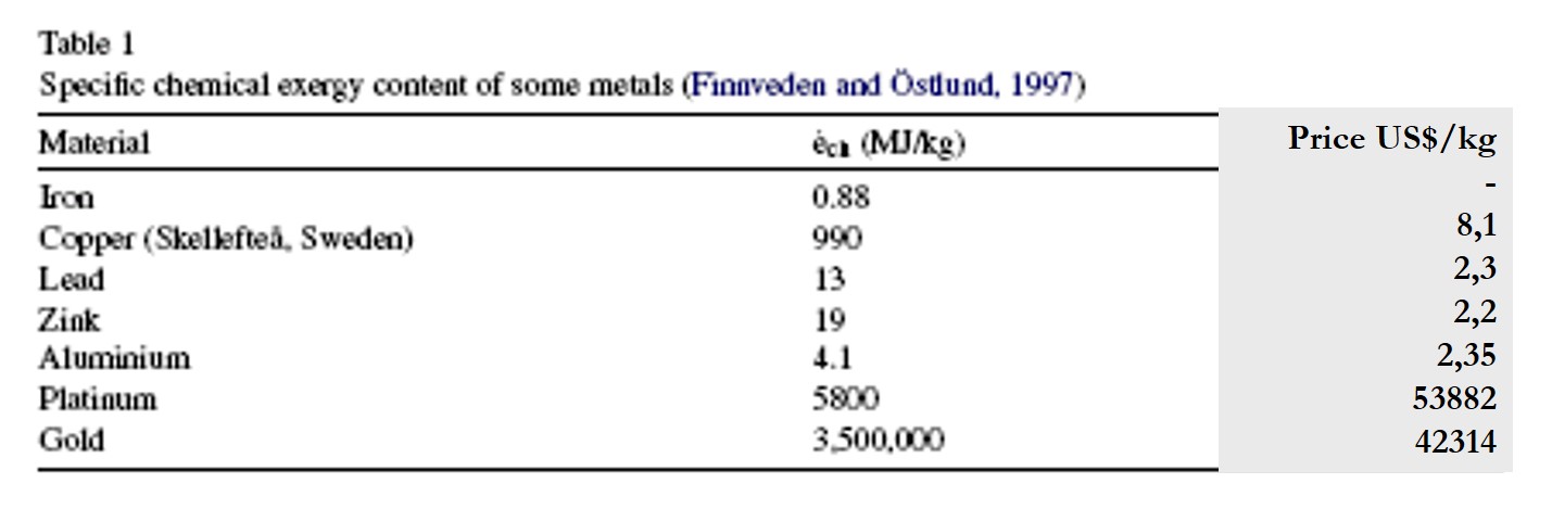
Ore concentration has an important relation with exergy content. The high-concentration lead deposits, for instance, have a chemical potential with respect to the average crustal abundance that gives them a non-zero exergy content. In other words, natural processes, fed by nuclear energy on the Sun and Earth, did the separating work we benefit from (Table 1).
It is possible to estimate the exergy content of ore presently mined. Some values are given in the Table below. The ore grades for these elements vary from less than 0,002 for Au and Pt to 4-5% for Pb, Zn and Cu to over 45% for Al. It illustrates the large work potential (exergy) these elements have in their pure form (the nature of the chemical bonding is another important determinant besides ore concentration). It makes also clear how important it is to promote recycling wherever possible and to prevent dissipation of these metals into (very) small concentrations.
Footnote
[1] Some elements in seawater get concentrated by natural processes, such as manganese (Mn) nodules on the ocean floor. Sometimes their increase is substantial on the scale of decades, which make such occurrences nearly a renewable resource. They are a prime example of common pool resources (CPRs) (§5.4).
Literature
H.J.M. de Vries, Effects of resource assessments on optimal depletion estimates. Resources Policy 15(3)19189 pp. 253-268
[1] Some elements in seawater get concentrated by natural processes, such as manganese (Mn) nodules on the ocean floor. Sometimes their increase is substantial on the scale of decades, which make such occurrences nearly a renewable resource. They are a prime example of common pool resources (CPRs) (§5.4).[/fusion_builder_column][/fusion_builder_row][/fusion_builder_container]
Leave A Comment