Energy Economics

Energy use: economics of energy saving

The dynamics behind the changes in energy intensity is an important topic in energy economics. Goods and services are produced with a variety of inputs and a so-called production function has been proposed to describe it. Engineers prefer to construct it on the basis of physical flows (engineering production functions), but this is difficult for all but a few basic processes (steel, cement and some others). Economists use an economic production function, in which the inputs of, notably, investments in capital stock K and operational inputs of labour L and energy E (and sometimes materials M) are expressed in monetary units. The problem of aggregation is then of course not easily resolved.

Following the usual simplification, a manufacturing plant produces P units/yr of a good with machinery valued as a capital stock K (€) and energy input E energy (GJ/yr) [1]. Labour is not considered. Energy use can be reduced by investments in, for instance, larger heat exchangers, waste heat recovery and so on. Such measures substitute capital for energy, which diminishes the energy required to produce the same output. A common formula for a production function is [2]:

       units/yr             (1)

A_t is the role of technology, assumed to be exogenous and productivity-increasing. For a constant reference output level P₀ at t=0, the unit costs are:

                                                     €/unit/yr          (2)

with c = C/P₀, p_i the price of factors i = K, E respectively and k = K/P₀, e = E/P₀ [3]. The formulation implies that an energy flow can be substituted with a capital stock. Any change in the p_E would induce a switch to a technology using less E and more K as long as the savings exceed the cost. In other words, as long as:

                                                             €/yr                  (3)

Assuming reference levels P₀ = 1 and A₀ = 1 and rewriting the production function gives:

€/unit              (4)

Inserting this in eqn. 2, one can plot c and k as a function of energy input e (Figure 1). The energy cost per unit are a linear function of the energy input with the (constant) energy price p_E as slope. The capital cost per unit are a downward sloping curve as a function of the energy input for a given (constant) capital ‘price’. The grey curve are the total costs at an energy price p_E = 1. It shifts to the black curve if the energy price rises to p_E = 10 at constant p_K. The arrow indicates the additional capital investment needed to operate at minimum unit cost at the higher energy price. The plant is then operated at higher fixed capital cost but lower operational (energy) cost and this ‘energy-saving’ operation makes the unit cost about ten units less costly than doing nothing (the grey curve). Reaching this ‘optimum’ implies cost rationality [4]. It can be proven that the minimum cost in the total cost curve is for .[5] It corresponds in engineering terms with, for example, a certain size of a heat exchanger surface, a certain thickness of insulation material or a certain number of steps in a distillation column.

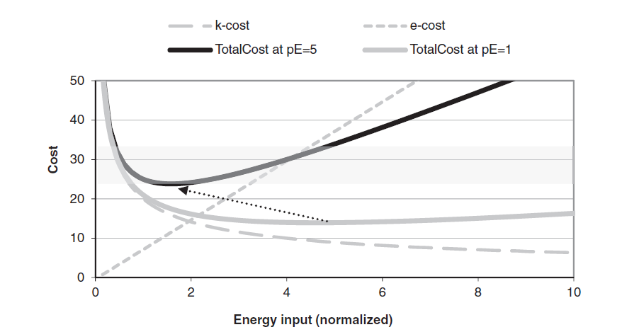
Figure 1. Substitution dynamics between capital and energy. The dashed curves indicate the per unit cost as function of the energy input (A₀ = 1, α = 0,5, p_K = 10 and p_E = 5). The upper dashed curve are total costs. The linear curve are energy costs. If pE goes up, the total cost and energy cost curves move upwards, and the minimum cost level will be at a lower energy input.

Manufacturers, as well as office managers and households, will often combine replacement investments with expansion investments. This makes it more difficult to find optimal estimates of DE and DK. In the practical evaluation of whether to switch from technology 1 → 2, often the simpler criterium of the payback time (PBT) is applied:

  yr         (5)

This rule-of-thumb investment criterium says that a firm will only decide to switch to a more energy-efficient technique if the ratio of additional investment and annually saved expenditures is less than PBT years. The lower PBT, the stricter is the criterium. The higher p_E, the more efficiency-investments are made.

Economists emphasize that this ‘simple’ model represents how ‘the market’ works – or should work. It offers two insights. First, it is the ratio of energy and capital price, not the energy price per se, that induces efficiency gains. If the price of capital p_K increases too, for instance because the investor can get a higher return elsewhere, then the reduction in energy use will be lower. This is one link between the energy and the financial sector. Secondly, the approach is ideal-typisch: it presumes that there is a continuous set of energy-savings options and that the firm operates on this production frontier (eqn. 1). In reality, there will be a discrete set of available techniques along this production frontier which are always ‘on the move’ in the K-E-plane because of (expectations about) innovations, energy prices, environmental regulation, changing tax regimes, wage negotiations and so on. Indeed, these options are partly autonomous (‘pure science’) and usually only developed when the energy price increases or is expected to do so (in the short term – markets are myopic). The term A_t is an insufficient proxy for all of this.

A second insight concerns different definitions of energy efficiency potentials. The theoretical potential is in physical terms and not in monetary terms determined by the laws of thermodynamics – it can never be realized (see www.sustainabilityscience.eu/energy-units-and-savings-dynamics). It is some vertical line to the left in Figure 1. Strictly speaking, one should, therefore, use a production function of the form . The technical potential at any given moment will rarely be realised, because it will run against the rising cost barrier and becomes too expensive. The economic potential is given by the optimal investment at the minimum overall cost, as outlined above.

Note that the cost curve in Figure 1 is the equivalent of a supply cost curve (SCC) in energy supply. Therefore, its empirical equivalent is called an efficiency supply cost curve (ESCC). The ESCC may fall over time when incremental innovations in the process of learning-by-doing bring down the production frontier and the economic potential approaches the technical potential. Innovation should be interpreted here in a broad sense: It refers to technical as well as organizational and legal skills, practices and measures. Even more important are technological breakthroughs, such as fundamental innovations that lift the technical potential, thus creating a new branch in production space. In some situations, the total cost curve is almost flat, which suggests that energy efficiency is possible at no additional costs. Such possibilities are called no-regret or win-win options. But the common situation is that, after the ‘low-hanging fruit’ has been picked, more efficient technologies and organisational measures are accompanied by higher cost.

 

Energy use in the macro-economy

Economists have introduced the economic production function in economic growth theory to. It is an aggregate representation of the production factors labour L and capital K. Labour – in essence: knowledge and organization, because most physical work has been substituted for by fuels and electricity – is usually the largest cost component. Capital, in the form of buildings, machinery and equipment, is an important second component. The cost of the inputs are called factor costs and equal to the total product value. The part made up by rewards for labour (wages, salaries) and for capital (dividends, rent) is the value added (VA). The existence and usefulness of this notion have been fiercely debated among economists since its inception in early 20^th century.  From a sustainability perspective, a key question is whether such a production function should not also include energy and materials and, perhaps again, land.

Until the oil crises of the 1970s, energy was not considered in economic analyses and neither were materials. It is understandable: coal and later oil and gas became ever cheaper in the industrial economy and were considered an operational input, not a potential constraint. The argument that energy and materials can be omitted in the production function because they are in most production processes only a rather small fraction of total factor costs, except for a few sectors such as mining and petrochemicals, seems no longer valid.

From a natural science perspective, it has been argued since the 1930s that energy inputs, if properly measured, are a key explanatory factor of economic growth. ”You cannot permanently pit an absurd human convention, such as the spontaneous increment of debt [compound interest], against the natural law of the spontaneous decrement of wealth [entropy].” (Soddy, in Cartesian Economics 1922:30). More recently, the role of energy and, particularly, exergy in economic production has been examined in detail. It appears that the inclusion of useful work (‘exergy services’) explicitly as an input in the production function yields an almost perfect correlation with GDP-growth for the period 1900-1975 (USA) and 1960-1993 (USA, Japan, Germany) (Warr et al. 2002; Kümmel et al. 2002, Ayres and Warr 2005) [6]. The analyses make it clear that useful work is a sine qua non for the growth in economic output realized in the high-income regions in the 20^th century and being underway in emerging economies in the 21^st century[7]. It strongly suggests that GDP-growth in the low-income regions of the world must concur with an increase in the use of exergy services, notably electricity. The apparent trend break around 1975 in the USA and other advanced economies is possibly explained by the oil price hike induced efforts to increase energy productivity and by the rise of ICT.

Since the 1980s, attempts are made to introduce energy and materials explicitly into the production function – the so-called KLEM-production function [8]. The results are, however, rather inconclusive due to the fact that energy can be both substitute and complement to labour and capital and that technological change is treated at too high an aggregation level.

Another approach has been the construction of an engineering production function. The practice of the industrial economy is strongly rooted in physical and chemical engineering and is characterized by cost-rationality, as discussed above. In subdisciplines such as engineering and business economics, industrial manufacturing processes are considered as a system that can be described by such an engineering production functions. It introduces explicitly physical inputs in the economic process and has therefore a rather solid empirical basis.

A problem with engineering production functions, however, is that they are specific for particular processes and for certain places and periods and that, particular in modern high-tech processes, there is a bewildering variety of energy and notably material inputs which are also difficult to aggregate even at constant prices.

Literature

Ayres, R., and B. Warr (2005). Accounting for growth: the role of physical work. Structural Change and Economic Dynamics 16 (2005) 181–209

Banks, F. (2000). Energy economics: A modern introduction. Kluwer Academic Publishers, Boston/Dordrecht/London

Blok, K., and E. Nieuwlaar (2020). Introduction to Energy Analysis. Routledge

Kümmel, R., J. Henn and D. Lindenberger (2002). Capital, labor, energy and creativity: modeling innovation diffusion.  Structural Change and Economic Dynamics 13(2002)415–433

Warr, A., H. Schandl and R. Ayres (2002). Long term trends in resource exergy consumption and useful work supplies in the UK, 1900 to 2000. Ecological Economics

Zweifel, P., A. Praktiknio and G. Erdmann (2017).Energy Economics: Theory and Applications. Springer International Publishing AG

 

Footnotes

[1] A similar function can be postulated for (operation of) a house or an office, with efficiency measures like more insulation and double glazing. It has also been postulated for the economy as a whole (macro production function). Such a high level of aggregation, however, gives interpretation problems. Besides, the empirical data have as yet given ambiguous confirmation of capital-labour substitution at the aggregate level of a sector or an economy. The reason is that capital and energy are not only substitutes but also, and certainly in a longer time perspective, complements – think of mechanization, automation or robotization).

[2] It is named after the economists who proposed it: Cobb and Douglas. A usual assumption is that there are no positive or negative effects on output from increase in scale (α + β = 1).

[3] Note that the input of energy per unit of output is the energy intensity (MJ/€).

[4] It is assumed that the additional investment Dk is depreciated over an economic lifetime of L years, that is: at a rate of Dk/L. The ‘price’ of the investment p_k can then be calculated in the form of an annuity, which includes depreciation and rent in the cost of capital.

[5] Of course, energy also substitutes for labour and environment, for instance in automation and pollution abatement. This makes the analysis more complicated.

[6] If commercial energy use is used for U instead of useful work, the correlation with empirical data is much weaker.

[7] Two other conclusions are that  electric power is of more than proportionate importance due to its high quality, and that there is a discrepancy between the elasticity of production and the cost shares of energy and labour. The latter points at the necessity of higher energy prices and lower labour costs/prices.

[8] With more pressure on land for food and biomass-based fuels, land may return as a production factor.