
Modelling catastrophic change
The simplest mathematical equation that represents bifurcations and catastrophic change is a first order differential equation of the form:

Solving for the attractors (dX/dt = 0), it is seen that one root is X = 0 and it represents a globally unstable attractor and the other two roots are for X* = ±√a. For a = 0, there is only one, unstable attractor. For a < 0, the roots are imaginary and the system exhibits oscillations. For a > 0, the two non-zero attractors are both locally stable (X = ± √a). This is seen in the phase plane for a = 4, 8 and 12 (Figure 1).
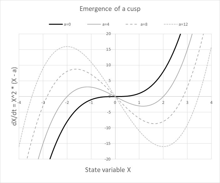 Figure 1 Phase space diagram for the first order differential equation 1. The solid line is for a = 0 in eqn. 1. The grey curves are for a = 4, a = 8 and a = 12: the larger a, the more outspoken the cusp.
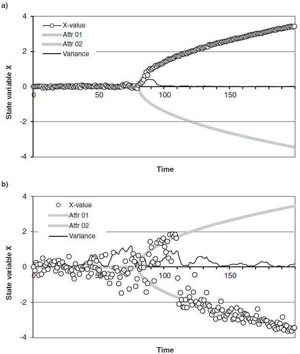
Figure 2 Bifurcation diagram. The dots indicate the state variable X according to eqn. 1, for a change of the slow variable a from −5 to +5 (Δt = 0,01, Runge-Kutta4). The grey curves are the attractor curves, with the cusp showing up at a = 0 (around t ~ 90). In the upper graph (a), the random fluctuation equals 0.2 and the system follows the upper path. In the lower graph (b), the random fluctuation is ten times higher (2) which causes the system to suddenly switch path for a ~ 1 (around t ~ 110). The thin lines are a measure of the variance.
Let the state variable X be the fast-changing variable. The system remains at the unstable attractor X = 0 for a = 0. For a > 0, the smallest perturbation from the state X = 0 will make the system move to one of the stable attractors (grey curves in Figure 1).
A simple simulation can clarify this. Suppose that a slow variable, represented by a in equation 2, changes in the course of a period of 100 quarters (25 year) from –5 to +5. During this change, the system will shift from one unstable attractor for a ≤ 0 to three (one unstable, two stable) attractors for a > 0 (upper graphs in Figure 2). The time-path of the state variable X will for such a slowly rising a start to move along one of the two grey attractor curves (lower graphs in Figure 2). The emergence of the fork at a = 0 is called a bifurcation. In three-dimensional X-a-space, it is a cusp.
If there are environmental noise or fluctuations in X, the system will for a = 0 simply fluctuate around the equilibrium at X = 0. As soon as the bifurcation emerges for a > 0, it depends on chance which of the two pathways is chosen. If the fluctuation is large relative to the separation of 2√a between the two branches, the system may start at one branch and then switch from one to the other one (lower graphs in Figure 2). As discussed elsewhere, the width of the attractor basin is a defining characteristic of resilience.
It is hard in this situation to derive firm statements about the present and future state of the system, because the stability landscape is rather flat in the neighbourhood of the bifurcation point. Environmental noise can therefore have a relatively large impact on X around this point. This is seen in the value of the variance during the simulation (right-hand graphs in Figure 2). Recent investigations suggest that careful analysis of the patterns of fluctuations over time may be an indicator of a critical transition (Biggs et al. 2009, Scheffer et al. 2009). Such ‘before-the-collapse’ signals may serve as an early warning indicator.
Tipping points
The sudden and not or difficult to reverse collapse in a system has been popularized under the name tipping points. The process of ‘tipping’ occurs when a system is forced outside the basin of attraction of the original equilibrium, after which it moves in a critical transition to an alternative, often less-desirable, stable state. In first instance, the notions of critical transitions and tipping points appeared in ecosystems research, where it was found that restring ecosystem health became surprisingly difficult once a certain ‘critical level’ of human interference was exceeded (see https://www.sustainabilityscience.eu/catastrophic-change/). The underlying idea of multiple attractors has also been proposed in order to understand dynamic changes in social, political and economic systems (e.g. Vries 1989, Scheffer 2009). Perhaps most widely known and discussed, it has been explored in relation to climate change. A seminal paper by Lenton et al. (2008) listed more than a dozen potential tipping points in the world climate system. Potential climate tipping points are an accelerated melting of Arctic sea-ice, a collapse in the Atlantic Ocean thermohaline circulation and a sudden disappearance of the Amazon forest. Some of these might already ‘tip over’ in this century. In the last decade, there has been an exponential increase in articles on climate tipping points.
There is an interesting debate going on between those scientists who argue that enough insights has been gathered to give a serious warning about such climate tipping points, and others for whom the empirical evidence from (eco)systems field research is not yet convincing enough. An example of the latter is the paper by Rietkerk et al. (2021), who argue that tipping points can be evaded through various pathways of spatial pattern formation. It would imply that complex ecosystems are more resilient that one would think on the basis of well-known but relatively simple models in mathematical ecology. Other research also points in this direction, for instance patches of bare ground surrounded by rings of tall grass – the god’s footprints’ in Namibia – can possibly be explained by an interaction between termites and plants (Pennisi 2017). Patterns emerge from the ‘territorial aggression’ interaction between insect populations and scale-dependent plant growth in a water-scarce environment. It is related to what has become known as self-organizing systems.
It contains a lesson one can also learn from system dynamics. In understanding and modelling complex (Earth) systems, one can think of a ‘ball-in-a-landscape’. The landscape has plains, mountain tops and valleys and, in this mechanical metaphor, the valleys can be interpreted as ‘attractors’. There are uncertainties at here at three levels:
- There may be attractors in the system which are (yet) unknown because they have not been manifest;
- The (human) intervention in the system can itself cause changes in the landscape; and
- There can be negative feedback mechanisms in the system which respond to the catastrophic change dynamic with novel, as yet hidden or non-existent processes..
The third uncertainty supposes an inherent resilience in (eco)systems. It is therefore safe to conclude that uncertainties about the pathways of large (eco)systems – for which controlled experiments are not possible – will persist. One should therefore be cautious with the interpretation of and communication about early warning signals.
Literature
Biggs, R., S. Carpenter and W. Brock (2009). Turning back from the brink: Detecting an impending regime shift in time to avert it. PROC. NATL. ACAD. SCI. (PNAS) 106(2009)826-831
Lenton, T., H. Held, E. Kriegler, and H.-J. Schellnhuber (2008). Tipping elements in the Earth’s climate system. PNAS 105(2008)1786-1793
Pennisi, E. (2017). Fairy circles could be the handiwork of hungry termites and thirsty plants. Science 18 january 2017
Rietkerk, M., R. Bastiaansen, J. van de Koppel, and A. Doelman (2021). Evasion of tipping in complex systems through spatial pattern formation. Science 8 oct 2021
Scheffer, M. (2009). Critical Transitions in Nature and Society. Princeton University, Princeton
Scheffer M, J. Bascompte, W. Brock et al. (2009) Early-warning signals for critical transitions. Nature 461:53–59.
Tarnita, C., J. Bonachela, E. Sheffer et al. (2017). A theoretical foundation for multi-scale regular vegetation patterns. Nature 541(2017)398-401
Vries, H. J. M. de (1989). Sustainable resource use – An enquiry into modelling and planning. PhD-thesis University of Groningen
https://decorrespondent.nl/15628/alarm-slaan-of-beter-bewijs-zoeken-de-wetenschappelijke-strijd-achter-kantelpunten-in-het-klimaat/170895a1-12c0-08f8-2aac-31974f1ec031#het-mysterie-van-het-verdwenen-kantelpunt
Leave A Comment