Measuring monetary flows: I-O matrices
National economic models have usually more sectors than the economic growth models discussed so far. Such sectoral disaggregation is based on a table or matrix of the intersectoral flows, or intermediate deliveries, between economic sectors: the input-output (I-O) table. They offer a bridge between the empirical data on monetary transactions on the one hand and the mechanisms behind economic growth on the other. From the I-O table it is immediately seen how much input from an economic sector j is used per unit of final demand output from sector i, in €/€. This is the direct intensity of that input – and the input can be energy, steel or whatever specific the table contains. If we choose as the input the expenditures on labour or capital (sector i), one can calculate the direct labour- and capital-intensity. Most material- and energy-intensive sectors have a rather low labour-intensity and a rather high capital-intensity, at least in the high-income regions where wages are high. Not surprisingly, you induce much more energy use when you buy for 100€ products from the chemical sector than when you spent it on childcare – 20 times more in the Netherlands in 2001. Those same 100€ generate 6 times more employment when spent on childcare as compared to chemical products.
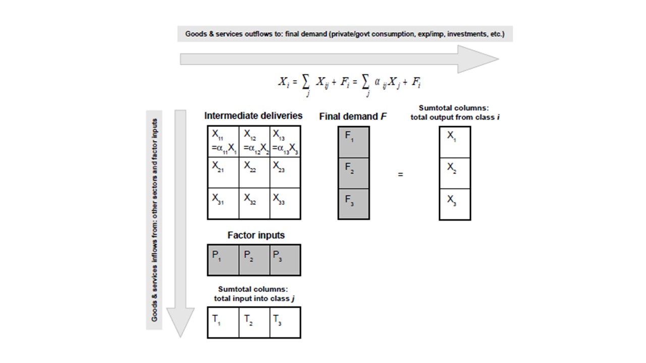
Input-output analysis was introduced by Leontiev in the 1940s. He arranged the transactions in an economy into three categories: deliveries to final demand, payments to primary inputs and net taxes, and intermediate deliveries between sectors. The latter are represented in a square matrix A, with the coefficients Aij indicating the monetary transactions between sectors i and j in the formal economy during a certain period, usually a calendar year, plus de column and row vectors of final demand and primary inputs [1]. The row vectors at the bottom are the payments for inputs to a sector, including the payments for the so-called primary production factors: wages for labour, dividends and interest for capital, and rent for land and other resources. The column vectors on the right are filled with the monetary outputs (or sales) to final demand, that is: to consumers, the government and exports minus imports. The sum of the column elements equals the sum of the row elements. GDP is defined as the value added (VA) in an economy which equals the summed rows of the primary inputs capital and labour. If I-O-tables have only a few sectors, much information remains concealed in the (large) diagonal elements of intrasectoral transactions. Lack of detail is because of lack of data and/or proprietary information.
Leontief introduced the assumption that the inputs are proportional to the outputs. In other words, the production function is a simple linear relationship between output Y and the limiting production factor K or L (Y = min[AK,BL] with A and B constants). The basic identity in an I-O table is:
![]() (eq. 1)
(eq. 1)
in an economy with n sectors and a final demand Fi for goods and services in sector I (Figure 1). It states that the output of any sector i equals the deliveries to all the other sectors and the deliveries to final demand. The assumption of a linear production function implies that the output Xi can be written as a linear function of the inputs Xij.
Figure 1. Scheme of an input-output (I-O) table (see above)
In words, each matrix element is divided by the sumtotal of the column elements. The elements αij = Xij/Xj are called the technical coefficients. For example, if sector j is the medical service sector and sector i is the electric power production sector, the ratio Xij/Xj = αij indicates the fraction of every € spent on medical services that is used to purchase electricity. An example of technical coefficients is given in Figure 2 (India 1998). It is seen that the Indian economy was then dominated by agricultural activity.
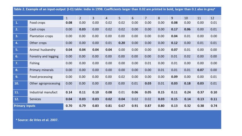
Figure 2 Technical coefficients for the economy of India in 1998 (de Vries et al. 2007).
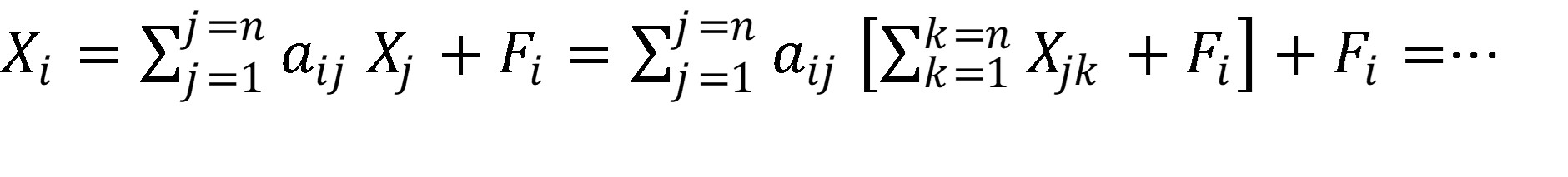
Inserting equation 2 into equation 1 and continue the substitution gives:
 (eq. 2)
In matrix notation, this becomes X = (I-A)−1 F, with I the identity matrix and A the coefficient matrix. The matrix A is a concise representation of the economic structure of a country.
I-O tables are used to calculate the monetary flows associated indirectly with a final demand output purchase, which yields the indirect intensity of a particular input. For instance, the energy used to deliver 1 kg of garbage bags has a direct energy-intensity αij with i energy sector and j bag manufacturer, but we can also calculate the energy used for the production of the plastic used in the bag (αjk with j plastic manufacturer and k bag manufacturer). The sum of direct and indirect intensity yields the total intensity. The differences in total intensities between sectors are smaller than the direct intensities. Take the example of childcare: part of your 100 € spent on childcare will be spent soon afterwards on gasoline by one of the employees travelling by car as part of her service sector job. This adds to the total energy-intensity.
An I-O matrix gives a static picture or snapshot of the structure of an economy. An extension is to introduce investment flows explicitly. Dynamic I-O-models isolate investments from the intermediate deliveries and make it part of final demand. In this way, the empirical data on structure can be combined with a standard economic growth model in order to simulate the system as it goes from one equilibrated situation at time t to the next at time t+Δt. During the transition, the technological coefficients are adjusted to represent trend- or expert-based expectations about (future) technologies (Wilting et al. 2008, Sassi et al. 2010).
Extensions and pitfalls
An extension is to disaggregate final demand in household categories and include also subsistence and informal transactions, also known as social accounting matrices (SAM). It is part of what is called structural economics. Such a disaggregation becomes important if one wishes to explicitly consider the role of households as key economic actors in civic society and their role as agents of social change. This is important for poor and rich countries alike, the more now that the welfare state is under pressure and self-reliance gets more priority. An example has been worked out for the EU, by classifying 17 household activities and 13 household types for 9 EU countries (Table 1; Duchin and Hubacek 2003). Such SAM’s can also help to include household and volunteer ‘work’ into economic statistics.
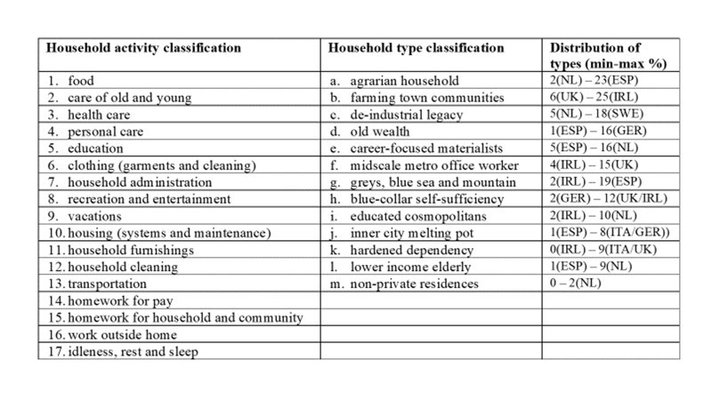
Table 1 Classification of household activity and type (Duchin and Hubacek 2003)
A further extension is to include more detail on the primary factor contributions, e.g. separating non-paid agricultural labour and various income classes. For low-income agrarian societies this is a more adequate framework than the monetary I-O table (Morrison and Thorbecke 1990).
One of the challenges in sustainability science is to connect economic growth models and input-output data in a transparent and effective way. Inputs of resources and ecosystem services are not valued until the moment that people add value by digging, transporting or any other form of processing; damage from pollution is only implicitly considered in the form of cleaning-up expenditures. To remedy this, the country-based economic input-output (I-O) tables are combined with so-called satellite accounts for natural resource stocks and flows and with trade statistics (Miller and Blair 2022). These represent I-O tables in physical flows and are sometimes called Physical Input-Output Tables (PIOT). The elements of the I-O-matrix are converted to physical units with use of (average) sectoral prices and double-checked with statistical data on physical flows.
A systematic connection between monetary and physical I-O stocks and flows was first applied in energy analysis. Later, environmental accounts were used to assess the sectoral origins of pollutants and the use of materials per unit of monetary final demand. In this way, the direct physical input (energy, material) and output (emission) flows associated with consumer and government expenditures can be calculated.
There are some pitfalls in the use of I-O-tables. One of those is how to deal with trade in open economies. An accurate treatment is to include the energy embodied in imports and in exports on the basis of transport and I-O tables for the trade partners. This is a rather tedious exercise. However, it can shed light on an element of unsustainability in globalization, namely that stricter environmental regulation in high-income regions makes it, in combination with cheap labour in low-income regions, profitable for corporations to move their (material- and energy-intensive) sectors away from high-income countries towards countries with less strict regulation. Theoretically, this is simply using a comparative cost advantage. Practically, it can lead to a slowdown or even decline in environmental and other regulation[2]. Analyses based on I-O-analyses with estimates of embodied energy in im/exports indicate that at least part of the dematerialization (in MJ/€) in the USA, Europe and Japan has occurred because of shifts in economic activity to Mexico, China and other low-income regions[3].
Literature
de Vries, B., A. Revi, G.K. Bhat, H. Hilderink and Pa.Lucas (2007). India 2050: scenarios for an uncertain future. MNP Report 550033002/2007, Bilthoven
Duchin, F., and K. Hubacek (2003). Liking social expenditures to household lifestyles. Futures 35(2003)61-74
Miller, R., and P. Blair (2022). Input-Output Analysis – Foundations and Extensions. Cambridge University Press, Cambridge
Sassi O., R. Crassous, J.-C. Hourcade, V. Gitz, H. Waisman, C. Guivarch (2010). Imaclim-R : a modelling framework to simulate sustainable development pathways. International Journal of Global Environmental Issues 10(2010)5–24
Wilting, H., A. Faber and A. Idenburg (2008). Investigating new technologies in a scenario context: description and application of an input-output method. Journal of Cleaner Production 16S1(2008)S102-S112
Foodnotes
[1] In network terminology, the economic sectors are the vertices and the transactions of buying from other sectors (input) and delivering to other sectors and to final demand (output) are the edges.
[2] The country with the lowest standards in environmental regulation – and other regulation, e.g. labour conditions and nature protection – attracts industries in search of higher profits and force other industries to lobby for less strict regulation in their country. This is the race-to-the-bottom dynamic.
[3] This is one of the aspects that complicate the negotiations about carbon-emission reductions in the context of international climate policy, because it invalidates a simple GJ/€ measure as indicator for emission targets.
Leave A Comment